1. Introduction
This work addresses the problem of a buyer and three suppliers. The suppliers present random lead-times under different statistical patterns; the first has a normal lead-time, the second a uniform distribution, and the third an exponential distribution. The goal is to define whether the orders should be made with the three suppliers or if this represents a wrong policy. The study aims to describe the order quantity and determine the reorder point that minimizes the inventory cost, complying with the established restriction of service level of 95%.
Inventories have been a subject of study for scholars and administrators since they are usually a significant amount of the company's assets, which is why they must be managed in such a way that they fulfill their function of having product availability at a reasonable cost, preferably the minimum, which is one of the objectives usually sought. The basic role of inventory is to absorb the differences between supply and demand for an item, which is often complicated by the uncertainty of the item's demand. When a company cannot know its demand with certainty, the resulting variations will be absorbed by the inventory because a shortage of materials could represent a loss of sales and a bad image for the company.
Inventory management involves two fundamental decisions: how much and when to place a new order.
Most inventory models seek one of the following objectives:
1. Minimize inventory management costs.
2. Maximize economic benefits, considering savings from purchasing larger volumes.
3. Maximize the internal rate of return on investment in inventories.
4. Define an inventory policy that is feasible and operational.
This study presents, for the first time, findings from scholars when several suppliers coexist to supply an order. An illustrative case solved by simulation is presented to show results and reach valuable conclusions about what should be done to optimize inventory costs.
Literature Review
Little research has been done when it comes to modeling a buyer's inventory with several suppliers and each of these with stochastic and diverse lead times, such as the present case study, in which there is cross-ordering, that is, when the buyer receives two orders in a row from the same supplier. The uncertainty of a product demand and the lead-times impact on establishing a larger safety stock has been proven previously. The safety stock and the inventory costs will increase if variability in these parameters is observed
| [1] | J. M. Izar, C. B. Ynzunza, A. Castillo, & R. Hernández, “Estudio comparativo del impacto de la media y varianza del tiempo de entrega y de la demanda en el costo del inventario,” Ingeniería, Investigación y Tecnología, vol. 17, no. 3, pp. 371-381, 2016. |
| [2] | F. Nasri, J. Paknejad, & J. F. Affisco, “Investing in lead-time variability reduction in a quality-adjusted inventory model with finite range stochastic lead-time,” Journal of Applied Mathematics and Decision Sciences, vol. 2008. No. 1, pp. 1-13, 2008. https://doi.org/10.1155/2008/795869 |
[1, 2]
.
A previous work
| [3] | D. Sculli, & S. Y. Wu, “Stock control with two suppliers and normal lead times,” Journal of the Operational Research Society, vol. 32, no. 11, pp. 1003-1009, 1981. https://doi.org/10.2307/2581854 |
[3]
estimated the mean and the distribution variance of a single item demand considering the lead-time of two different suppliers. Both lead-times are normal and two different orders are placed (one for each supplier). Their results established that the reorder point to avoid shortages is lower if both suppliers are used simultaneously, and the minimum order sizes in these circumstances were defined. Other scholars presented the optimal ordering policy when two suppliers have stochastic lead times and demands
| [4] | H. S. Lau, & L. G. Zhao, “Optimal ordering policies with two suppliers when lead times and demands are all stochastic,” European Journal of Operational Research, vol. 68, no. 1, pp. 120-133, 1993. https://doi.org/10.1016/0377-2217(93)90080-7 |
[4]
. This policy defines three issues: the order quantity, the reorder point, and the order proportion to each supplier. Among their findings are: (1) by splitting the orders, the inventory cycle cost is reduced, with the decrease in safety stock being a less relevant issue; (2) the lowest cost is achieved if the average lead-time of the second supplier is greater than the first; and (3) the optimal proportion of the order from each supplier varies with the difference in the average values of their lead-times. More recently
| [5] | S. M. Disney, A. Maltz, X. Wang, & R. D. Warburton, “Inventory management for stochastic lead times with order crossovers,” European Journal of Operational Research, vol. 248, no. 2, pp. 473-486, 2016. https://doi.org/10.1016/j.ejor.2015.07.047 |
[5]
, the impact of stochastic lead times with cross-ordering on inventory costs and safety stocks in a fixed-time variable order quantity (Out-Up-To (OUT)) ordering policy system was analyzed. They considered global logistics data that violated the traditional assumption of normal leadtime demand. They also found that cross-ordering is a common and important phenomenon in real supply chains. Therefore, a new method for determining the distribution of the number of open orders is presented. This method allows an accurate safety stock calculation for the so-called Proportional-Out-Up-To (POUT) policy, a popular, implementable, and linear generalization of the OUT policy. They claim that the OUT-replenishment policy is not cost-optimal in global supply chains since it can be shown that the POUT policy always outperforms when there is cross-ordering. The study showed that, unlike the constant lead-time case, minimum safety stocks and minimum inventory variation do not always lead to minimum costs under stochastic lead-times with cross-ordering. Other researchers
| [6] | J. C. Hayya, T. P. Harrison, & X. J. He, “The impact of stochastic lead time reduction on inventory cost under order crossover,” European Journal of Operational Research, 211(2), pp. 274-281, 2011. |
[6]
analyzed the impact on inventory cost of a reduction in a supplier lead-time when there is cross-ordering. Through exponential lead-times, the reduction in average leadtime has a secondary reduction in variance due to cross-ordering. The main objective is to reduce the inventory cost; if this offsets the investment in a lead-time reduction, then this strategy is advisable. Stolyar and Wang
| [7] | A. L. Stolyar, & Q. Wang, “Exploiting random lead times for significant inventory cost savings,” Operations Research, vol. 70, no. 4, pp. 2496-2516, 2022. https://doi.org/10.1287/opre.2021.2129 |
[7]
analyzed a single-item inventory system where unmet demands accumulate. Lead-times are random, independent, and identically distributed, causing orders to cross over time. They developed a new inventory policy to enhance the random lead time implications and the cross-ordering; its performance was evaluated using asymptotic analysis and simulations. Their ideology does not follow the basic principle of the Constant Base Stock (CBS) policy, or more generally, the (s,S) and (R,Q) policies, which is to keep inventory within a fixed range. Instead, it uses the current inventory level (inventory on hand minus backlog) to set a dynamic target for inventory in transit and place orders to meet this target. They demonstrate that following this policy, the average inventory cost can be significantly reduced compared to the CBS policy.
Optimal (R, Q) replenishment policies for stochastic inventory models for both the no-crossover case and the no-output case were developed
| [8] | A. Srivastav, & S. Agrawal, “On a single item single stage mixture inventory models with independent stochastic lead times,” Operational Research, vol. 20, no. 4, pp. 2189-2227, 2020. https://doi.org/10.1007/s12351-018-0408-z |
[8]
. Stockout costs are considered, the total cost expressions are developed for both cases, and their convexities are evaluated. A normal approximation method is used to determine the distribution of the lead time demand. The effect caused by the changes in the mix of backorder proportions and the sales lost on various inventory performance measures, such as total cost, service levels, and turnover ratio, is studied.
In addition, alternative methods for reducing the lead time and their impact on the safety stock and the inventory cost in a continuous review system (Q,s) were studied. It focuses on a single-supplier, single-buyer integrated inventory model with stochastic demand and a variable lead time that depends on the lot size, and the lead time consists of production, setup, and transportation time. The leadtime can be reduced by decreasing the setup and the transportation time, increasing production rate, or reducing lot size. It was confirmed that reducing lead time is especially beneficial in cases of uncertain demand. Furthermore, the combination of reducing the preparation and production time will automatically reduce costs
| [9] | C. H. Glock, “Lead time reduction strategies in a single-vendor–single-buyer integrated inventory model with lot size-dependent lead times and stochastic demand,” International Journal of Production Economics, vol. 136, no. 1, pp. 37-44, 2012. https://doi.org/10.1016/j.ijpe.2011.09.007 |
[9]
. Moreover, in the case of a single buyer and multiple heterogeneous suppliers, to make an adequate selection and to define the order size that minimizes the cost of the system is evaluated. In this study, the combinations of suppliers to reach the optimal solution are reduced, and the efficiency of the supply chain is increased using heuristic tools
| [10] | C. H. Glock, “A Multiple-vendor single-buyer integrated inventory model with a variable number of vendors,” Computers & Industrial Engineering, vol. 60, no. 1, pp. 173-182, 2011. https://doi.org/10.1016/j.cie.2010.11.001 |
[10]
.
Other researchers
| [11] | C. H. Glock, & T. Kim, “Shipment consolidation in a multiple-vendor-single-buyer integrated inventory model,” Computers & Industrial Engineering, no. 70, pp. 31-42, 2014. https://doi.org/10.1016/j.cie.2014.01.006 |
[11]
present a batch shipment program with one buyer and multiple sellers in which they must consolidate their shipments to reduce transportation costs. Large shipments must be shipped before small shipments, and suppliers with greater production capacity must occupy the last places in the shipment cycle. Also, a base stock policy to replenish inventories with an external supplier with a fixed lead time has been considered by a company that faces the Poissonian demand
| [12] | T. Ahmadi, Z. Atan, T. de Kok, & I. Adan, I. “Optimal control policies for an inventory system with commitment lead time,” Naval Research Logistics (NRL), vol. 66, no. 3, pp. 193-212, 2019. https://doi.org/10.1002/nav.21835 |
[12]
. A pre-order strategy that allows customers to place their orders ahead of their actual needs is implemented. The time from a customer's order to the date the product is needed is called the commitment lead time, for which the company pays a cost. The commitment unit cost threshold increases with unit holding and backorder costs and decreases with average lead-time demand. Also, the optimal solution of an inventory model for an integrated buyer-seller system with normal distribution of lead time was found
| [13] | M. A. Hoque, “A vendor–buyer integrated production–inventory model with normal distribution of lead time,” International Journal of Production Economics, vol. 144, no. 2, pp. 409-417, 2013. https://doi.org/10.1016/j.ijpe.2013.02.019 |
[13]
; for example, a triangular distribution for both demand and lead time was explored for a new product system
| [14] | P. Wanke, H. Ewbank, V. Leiva, & F. Rojas, “Inventory management for new products with triangularly distributed demand and lead-time,” Computers & Operations Research, vol. 69, no. C, pp. 97-108, 2015. https://doi.org/10.1016/j.cor.2015.10.017 |
[14]
.
Forecasting lead-time demand is the backbone of inventory control. Although multiple studies have been done on forecasting mean lead time demand, less research is available on forecasting its variation of stochastic lead-times. This represents a major gap in the literature since safety stock calculations are explicitly based on the lead time demand variance. Some scholars
| [15] | Z. Babai, D. Yong, L. Qinyun, A. Syntetos, & W. Xun, “Forecasting of lead-time demand variance: Implications for safety stock calculations,” European Journal of Operational Research, vol. 296, no. 3, pp. 846-861, 2022. https://doi.org/10.16/j.ejor.2021.04.017 |
[15]
close this gap by exploring the feasibility of three strategies to estimate the variance of the forecast error of this lead time demand: (1) adding the per-period variance of the forecast errors (most used); (2) considering the variance of the aggregate forecast error; and (3) contemplating the variance of the forecast errors resulting from the temporally aggregated demand. Their results show that the conventional strategy is the least accurate, except in cases of high negative demand autocorrelation. If such autocorrelation is positive, the classical strategy leads to higher inventory costs and lower service levels.
On the other hand, a base stock inventory system for perishable products with Markovian demand and general distributions of lead time and shelf life is being investigated.
| [16] | C. Kouki, B. Legros, J. Z. Babai, & O. Jouini, “Analysis of base-stock perishable inventory systems with general lifetime and lead-time,” European Journal of Operational Research, vol. 287, no. 3, pp. 901-915, 2020. https://doi.org/10.1016/j.ejor.2020.05.024 |
[16]
. By using a queuing network model, explicit expressions of the stationary distribution of the inventory status were developed along with the expected total cost in a base stock system with lost sales. The main objective was to identify the substantial errors made when assuming deterministic or exponential distributions over time, which emphasizes the need to obtain results beyond these assumptions.
A research group analyzes supply planning and inventory control of perishable goods with uncertain lead times and service level constraints to determine the optimal replenishment quantity based on the remaining shelf life of the goods in the inventory, lead time demand forecasting, and inventory policy
| [17] | S. Transchel, & O. Hansen, “Supply planning and inventory control of perishable products under lead-time uncertainty and service level constraints,” Procedia Manufacturing, no. 39, pp. 1666-1672, 2019. https://doi.org/10.1016/j.promfg.2020.01.274 |
[17]
. In addition, they show the impact of not considering lead time uncertainty in decision-making to achieve a target service level. Based on the intensification of time-based competition, the importance of reducing lead time through the fast delivery of multiple orders in the replenishment-storage-transport process has been emphasized. This perception has led companies to increase their spends on modern time-tracking technologies (e.g., RFID) and equipping facilities for rapid item movement (e.g., high-bay automated racking) to retain customers. Also, a novel extension of the multi-item joint replenishment problem (JRP) with lead-time reduction initiatives was explored
| [18] | L. Cui, J. Deng, R. Liu, D. Xu, Y. Zhang, & M. Xu, “A stochastic multi-item replenishment and delivery problem with lead-time reduction initiatives and the solving methodologies,” Applied mathematics and computation, vol. 374, 125055, 2020. https://doi.org/10.1016/j.amc.2020.125055 |
[18]
. By assuming a controllable lead-time, a periodically reviewed stochastic joint replenishment and delivery (JRD) model was designed. This model investigates the impacts of capital investment in decreasing lead time on multi-item joint replenishment and delivery decisions. To solve the proposed JRD, two heuristics and a differential evolutionary algorithm based on the model property analyses are presented. Results reveal the performance differences (e.g., search speed, robustness, and search efficiency) of the three algorithms. These findings have managerial implications; a suitable investment in lead time reduction not only helps to shorten the replenishment time and reduce important ordering costs but can also reduce the system cost.
The lead-time flexibility in a two-stage continuous review supply chain, where the retailer uses the (R, Q) inventory system, is analyzed
| [19] | M. Çakanyildirim, & S. Luo, “Stochastic inventory system with lead time flexibility: offered by a manufacturer/transporter,” Journal of the Operational Research Society, no. 68, pp. 1533-1552, 2017. |
[19]
. Results show that when its inventory position reaches R, a new order of size Q is placed with the manufacturer, who uses a transportation provider to deliver it with different lead-time options. According to the contract, the manufacturer can accelerate or postpone the delivery if the retailer requests it. Therefore, the retailer has the flexibility to change the lead time using the most recent demand information. Sensitivity analysis shows that R is more sensitive to the change of the lead-time than Q; therefore, the paper mainly focuses on finding the optimal R. The order crossover problem is also analyzed, and an upper bound for the probability of this crossover is derived. Finally, the effects of lead time flexibility on supply chain performance are illustrated. On the other hand, a single product was studied to analyze a two-source inventory system with Poissonian demand and allowing for delays
| [20] | J. S. Song, L. Xiao, H. Zhang, & P. Zipkin, “Optimal policies for a dual-sourcing inventory problem with endogenous stochastic lead times,” Operations Research, vol. 65, no. 2, pp. 379-395, 2017. https://doi.org/10.1287/opre.2016.1557 |
[20]
. Inventory can be replenished through a normal supply source, which consists of a two-stage queue with exponential production time at each stage. It is also possible to place an emergency order by bypassing the first stage and paying a fee for it. There is no fixed cost per order. There are linear costs of ordering, holding, and back-ordering. Through a novel approach, they derive optimal ordering policies and characterize quasi-optimal heuristic policies.
Another researcher
| [21] | H. J. Lin, “Investing in lead-time variability reduction in a collaborative vendor–buyer supply chain model with stochastic lead time,” Computers & Operations Research, no. 72, pp. 43-49, 2016. https://doi.org/10.1016/j.cor.2016.02.002 |
[21]
deals with investment in reducing lead time variability for the integrated supplier-buyer supply chain system with partial lag under stochastic lead time. It is considered that the lead-time variability can be reduced by an increased investment; more specifically, a logarithmic investment function is used, which allows investments to reduce lead time variability. By using this supply chain model, considerable savings are achieved to increase competitive advantages. The goal is to derive the optimal production/ordering strategy and the best investment policy to minimize the total joint cost.
Time-based competition has attracted significant attention since the 1980s. Supply chain managers have tried various approaches to improve their performance by reducing lead-time and its variance. The lead time reduction in batch-order inventory policies under reorder points has been explored and quantified
. Instead of using approximate total cost equations, an exact total cost equation that is based on an inherent relationship between on-hand inventory and backorders is presented. Therefore, the analysis of the marginal value of lead-time and its variance achieves more accurate results. The analytical results show that inventory cost is a strictly increasing concave function of the lead-time and its variance. In other words, the cost savings in both decreases as the lead-time increases. These cost savings are also shown to increase linearly with the rate of the inventory carrying cost. When the variation coefficients of the demand and lead-time are exceedingly small, the variation of the lead time is imperative; otherwise, the focus should be on reducing the lead-time.
A stochastic inventory model to determine the optimal reorder point and order quantity was explored
| [23] | M. A. Alam, Z. Hasan, S. A. Siam, A. K. M. T. Abedin, & N. A. Habib, “Inventory Cost Optimization with Normally Distributed Lead Time and Stochastic Demand Considering Fill Rate,” International Journal of Scientific & Engineering Research, vol. 8, no. 12, pp. 1284-1291, 2017. https://doi.org/10.14299/IJSER.2017.12.009 |
[23]
. A hybrid equation of total inventory cost in which customer demand is deterministic at reordering time and after the reorder point was developed. The order quantity Q and reorder point R were determined by different equations. In the traditional economic order quantity (EOQ) model, the inventory carrying cost is the most expensive. But in this hybrid model, a penalty cost is included related to the fill rate.
Regarding the information technology (IT) sector, it is common to contract a single supplier; however, it is becoming increasingly popular to split the IT services between several suppliers
| [24] | S. Handley, K. Skowronski, & D. Thakar, “The single‐sourcing versus multisourcing decision in information technology outsourcing,” Journal of Operations Management, vol. 68, no. 6-7, pp. 702-727, 2022. https://doi.org/10.1002/joom.1174 |
[24]
. The trend towards using multiple suppliers illustrates a broader movement towards greater disaggregation and knowledge distribution. Their results show that abroad suppliers with more experience are less likely to establish multiple contracting arrangements.
Recent studies
| [25] | X. Chen, J. Lyu, S. Yuan, & Y. Zhou, “Learning in Lost-Sales Inventory Systems with Stochastic Lead Times and Random Supplies,” (December 21, 2023). http://dx.doi.org/10.2139/ssrn.4671416 |
[25]
have considered the problem of managing lost-sales inventory systems with general supply uncertainty (stochastic lead times and random supplies), if the decision maker has no prior information on stochastic demand and supply. They propose the first effective learning algorithm for inventory management problems with censored demand and supply data under general supply uncertainty.
Other researchers
| [26] | O. Hansen, S. Transchel, & H. Friedrich, “Replenishment strategies for lost sales inventory systems of perishables under demand and lead time uncertainty,” European Journal of Operational Research, vol. 308, no. 2, pp. 661-675, 2023. https://doi.org/10.1016/j.ejor.2022.11.041 |
[26]
developed an inventory control policy for perishable products considering random demand and random lead time, considering that excess demand is lost. The policy dynamically determines the optimal replenishment quantity under a service level constraint in every period, allowing for order-crossing, a widely disregarded characteristic in the literature. They compare the two most extreme issuing policies, first-expired-first-out (FEFO) and last-expired-first-out (LEFO), and evaluate our policy to existing inventory policies for perishables that typically ignore lead time uncertainty. They show that ignoring lead time uncertainty and planning based on the expected lead time significantly undershoots the target service level. Under LEFO, the service level achieved would still fall considerably below the target, which the lost-sales structure can explain. On the other hand, under FEFO, the service level achieved would overshoot the target service level, which leads to unnecessary waste. A more reliable lead time can significantly reduce waste, especially under LEFO.
Yuan et al. consider the lost-sales inventory systems with stochastic lead times and establish the asymptotic optimality of base-stock policies for such systems
| [27] | S. Yuan, J. Lyu, J. Xie, & Y. Zhou, “Asymptotic optimality of base-stock policies for lost-sales inventory systems with stochastic lead times,” Operations Research Letters, 57, 107196, 2024. https://doi.org/10.1016/j.orl.2024.107196 |
[27]
. They prove that as the per-unit lost-sales penalty cost becomes large compared to the per-unit holding cost, the ratio of the optimal base-stock policy's cost to the optimal cost converges to one.
Another study
| [28] | J. Wang, Y. Fu, J. Zhou, L. Yang, & Y. Yang, “Condition-based maintenance for redundant systems considering spare inventory with stochastic lead time,” Reliability Engineering & System Safety, 257, 110837, 2025. https://doi.org/10.1016/j.ress.2025.110837 |
[28]
focuses on joint optimization problems to minimize the total cost rate considering stochastic maintenance time for components and stochastic lead time for spares. The problem is modeled as a Markov decision process model and solved by an improved reinforcement learning algorithm, i.e., the improved Q-learning algorithm, which converges more quickly and reaches a smaller value of the total cost rate than the traditional Q-learning algorithm.
Materials and methods
The order quantity, Q, and the reorder point, R, were calculated through simulation minimizing the inventory cost. These costs include the cost of placing new orders (Cord), the cost of maintaining the inventory (Cmai), and the cost of shortages when necessary (Csho).
The equation for the cost of placing orders is:
Where:
Cord = Cost of placing inventory orders, $/period
Co = Cost of each order, $/order
Since it is a daily period problem, it needs to be calculated when a new order is placed. The maintenance cost is given by the following mathematical expression:
Cmai=Cm(AverageInventory)(2)
Where:
Cmai = Cost of inventory maintenance, $/period
Cm = Cost of maintenance of each item, $/unit
The average inventory is obtained depending on how the simulation is done. This study considers a calculation per day, so the daily average is reported.
On the other hand, the cost of shortages is obtained with the following equation:
Where:
Csho = Cost of shortages, $/period
Cs = Cost of each shortage, $/unit
Ns = Number of shortages, units/period
The cost of each shortage is expressed by the lack of items in the inventory, in this case, the difference between the price and the cost of the item. The total cost is the sum of the previous three to vary the order quantity, Q, and the reorder point R, with which the minimum cost is obtained.
In addition, the restriction on the service level is considered, which must be greater or equal to 95%.
The service level (sl) is defined as follows:
sl=1-(Timesthatshortagesappear)/(Numberoforders)(4)
The simulation in Excel taking random values for the probabilistic variables like product demand and the lead times of the three suppliers is conducted to determine the values of Q and R that minimize the total inventory cost.
Case Study
An item with average demand, with a mean of 650 units per day and a standard deviation of 230 is considered. This product is provided by three different suppliers with the same average lead time. The first case presents a normal lead-time with a mean of 8 days and a standard deviation of 3 days; the second supplier with a uniform distribution between 4 and 12 days lead-time; and the third supplier with an exponential lead-time with a mean of 8 days. The cost of placing each order for the three suppliers is $ 12,000, and the price per item is $220 with a sale price of $480; therefore, the cost of each shortage is $ 260 (the difference between these two amounts). It is assumed that each time a new order is placed, one-third of it is placed with each supplier. The cost of keeping each item in inventory is $1.45/day. There is a restriction on the service level, which must be greater than or equal to 95%. The study aims to determine if the policy of using three different suppliers, requesting the same volume from each one, is advantageous or should be modified.
2. Results
A daily period is defined for the simulation, which starts the first day (order quantity Q) and the inventory decreases daily according to the normal demand following the next equation:
Where µ is the mean and σ the standard deviation of the demand, while X is a random number obtained in Excel to estimate the item demand.
The probabilistic lead-time of each order for the first supplier (L1) which is normal, is given by the following mathematical expression:
Where µL is the mean, σL the standard deviation of the normal distribution of the lead-time of the first supplier, and X is a random number obtained in Excel.
The lead-time of the second supplier (L2) is obtained with the following equation:
Where a and b are the upper and lower limits of the uniform distribution and X is another random number.
The lead-time of the third supplier (L3) is exponential and is calculated with the equation:
Where µE is the average lead-time of the third supplier and X is another random number.
The average inventory holding cost is estimated daily and the other expenses are determined by event, whether it is placing a new order or if shortages appear. The simulation is conducted with several runs and the annual cost is calculated, which is tested for different combinations of Q and R values.
If the reorder point is calculated traditionally, the lead time of the three suppliers would be 5,478 units.
For this initial case, called the base case, and considering the aforementioned data, the minimum cost is achieved with a Q of 12,000 items per order and a reorder point R of 9,000 units, with a service level of 95.6% and a total cost of $5,210,200/year, of which $194,600 are for making new orders, $4,179,100 for inventory maintenance, and $836,500 for shortages. Based on the original case, a sensitivity analysis is performed, varying the fraction supplied by each supplier. The standard deviation of the lead-time of supplier 1 and the limits of the lead time of supplier 2 were modified without changing their average value and varying only their standard deviation. These modifications show how these changes may impact the inventory cost. For the third supplier, the standard deviation of lead-time was not modified due to its exponential pattern where the mean is equal to the standard deviation impacting the inventory cost to a greater extent.
In the first case, the fraction supplied by each supplier is modified considering the data of the base case, in which each supplier supplies a third of the order quantity (Q) or a single supplier provides everything. Results are shown in
Table 1, the values of Q and R to achieve the minimum cost are included.
Table 1. Inventory costs as the fraction provided by each supplier varies.
Supp. Frac. 1 | Supp. Frac. 2 | Supp. Frac. 3 | Q, units/order | R, units | Cost, M$/year |
0.333 | 0.333 | 0.333 | 12,000 | 9,000 | 5,210.2 |
1 | 0 | 0 | 12,700 | 9,000 | 4,961.2 |
0 | 1 | 0 | 13,300 | 9,000 | 5,699.2 |
0 | 0 | 1 | 23,000 | 16,000 | 10,849.9 |
0.5 | 0.25 | 0.25 | 13,000 | 9,500 | 5,442.9 |
0.25 | 0.5 | 0.25 | 13,300 | 9,500 | 5,431.0 |
0.25 | 0.25 | 0.5 | 13,500 | 9,200 | 5,847.9 |
0.4 | 0.4 | 0.2 | 14,000 | 8,500 | 5,107.2 |
0.4 | 0.2 | 0.4 | 14,000 | 8,500 | 5,146.2 |
0.2 | 0.4 | 0.4 | 13,600 | 9,500 | 5,673.2 |
Source: Author.
A multiple regression analysis was performed considering the fractions provided by each supplier as independent variables and the inventory cost as the dependent variable. The adjustment was statistically significant since the statistic F was 9.0036 with a pi value of 0.012 and the square R 0.7201, being the regression equation as follows:
Cost=9,373.3–5,535.74f1–4,473.45f2(9)
The cost is expressed in thousands of pesos per year, and f1 and f2 are the fractions provided by suppliers 1 and 2, respectively.
The fraction of supplier 3 was not included in the equation, since its beta coefficient resulted in a value of zero, which shows that it is the least relevant for the regression adjustment. The supplier fraction that contributes the most to reducing the cost is the first supplier; for every 1% increment in the fraction, the expense decreases by 55,360 pesos, while for the second supplier, the decrease is only 44,730 pesos.
The table above shows that point 4 presents a significantly higher cost when the entire order is supplied by the third supplier, which practically doubles the expense. On the other hand, the points with the lowest cost were the first (where each supplier supplies a third of the order), the second (where the entire order is provided by the first supplier), the eighth (where the first and second suppliers each provide 40% and the rest by the third supplier), and the point 9 (where the order is provided 40% by suppliers 1 and 3 and the remaining 20% by supplier 2). Overall, the minimum cost point was the second (less than five million pesos per year), where the entire order was supplied by the first provider.
The order quantity varies in 9 of the 10 points between 12,000 and 14,000 units per order. The only point that increases significantly, presenting a value of Q of 23,000 units per order, is the fourth, where the order is provided by the third supplier. On the other hand, the reorder point varied between 8,500 and 9,500 units, except for point 4, where the entire order is supplied by the third supplier resulting in 16,000 units.
The case runs with an average of 17 orders per year presenting some order crossovers, being the most frequent in the case of the third supplier. Its lead-time is exponential with an average of 3 crossovers per year. The second supplier shows a uniform distribution with an average of one crossover per year. The least frequent is the first supplier with a normal lead-time with an average of 0.5 order crossovers per year.
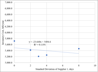
Table 2 shows the outcome of the changes in the base case by modifying the standard deviation of the lead time of supplier 1, whose pattern is normal. Q and R change in a narrow range, Q between 12,000 and 13,500 units per order and R between 9,000 and 9,800 units.
Table 2. Inventory cost when changing the standard deviation.
Lead-time Std. Dev., days | Q, units/order | R, units | Costo, M$/year |
0 | 12,300 | 9,800 | 5,722.7 |
2 | 13,000 | 9,200 | 5,418.8 |
3 | 12,000 | 9,000 | 5,210.2 |
4 | 13,000 | 9,200 | 5,253.4 |
8 | 13,500 | 9,500 | 5,465.9 |
Source: Author.
Figure 1. Inventory Cost as a Function of Supplier 1 Standard Deviation.
Figure 1 shows the standard deviation of the lead time of supplier 1, where the cost of the standard deviation is between zero and 3 days, contrary to what is expected. The behavior changes as the cost increases directly with the deviation from 3 to 8 days. The graph shows a square R of 0.119 and a negative slope indicating an inverse relationship between the cost of inventory and the standard deviation of the lead-time.
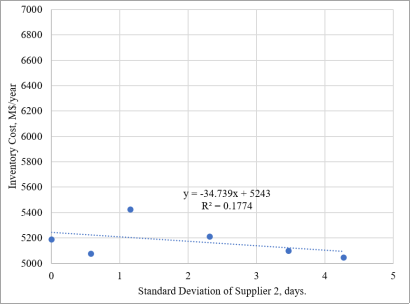
The change in the inventory cost was analyzed with the standard deviation of the lead-time of supplier 2, keeping its mean constant at 8 days. The results are summarized in
Table 3.Table 3. Change in inventory cost with standard deviation of supplier 2 lead time.
Std. Dev. Lead-time, days | Q, units/order | R, units | Costo, M$/year |
0 | 13,500 | 9,000 | 5,190.0 |
0.5774 | 13,800 | 8,700 | 5,076.2 |
1.1547 | 13,000 | 9,500 | 5,426.0 |
2.3094 | 12,000 | 9,000 | 5210.2 |
3.4641 | 12,500 | 8,500 | 5,098.3 |
4.2724 | 12,500 | 8,500 | 5,048.3 |
Source: Author.
Data shows that the cost does not increase directly with the standard deviation of the second supplier's lead-time. It reaches a maximum value at an intermediate level of the range of values studied for the standard deviation. The order quantity Q has fluctuated between 12,000 and 13,800 units per order, and the reorder point is between 8,500 and 9,500 units.
Figure 2 presents the change in the inventory cost, demonstrating a poor linearity and a negative slope, reflected in an inverse relationship between the expense and the standard deviation.
Figure 2. Inventory Cost as a Function of Supplier 2 Standard Deviation.
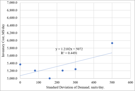
Table 4 includes the results when the standard deviation of the demand changes from the base case including the values of Q and R that lead to the optimal cost. Q has varied over a wider range, between 12,000 and 17,000 units per order, while R occurs between 8,000 and 9,000 units.
Table 4. Change in inventory cost with demand standard deviation.
Demand Std. Dev., units/day | Q, units/order | R, units | Costo, M$/year |
0 | 13,500 | 9,000 | 5,369.6 |
80 | 14,000 | 8,500 | 5,207.3 |
160 | 14,500 | 8,000 | 5,004.1 |
230 | 12,000 | 9,000 | 5,210.2 |
300 | 15,000 | 8,500 | 5,244.1 |
500 | 17,000 | 9,000 | 5,933.7 |
Source: Author.
Figure 3 graphically shows the change in the inventory cost, which is not linear. On the left side, a decrease in expense is observed with an increase of the standard deviation until reaching the minimum cost point (deviation of 160), and from there, the cost increases directly with the deviation. Similar to the other cases, poor linearity and a negative slope occur not allowing to establish a statistically significant relationship between the variables.
Figure 3. Inventory Cost Variance with Demand Standard Deviation.
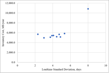
The inventory cost as a function of the standard deviation of lead-time is presented in
Figure 4, where it can be observed that there is where no defined pattern of variation is observed, except when the entire order is supplied by the third supplier (exponential lead-time), and the cost was almost doubled.
Figure 4. Inventory Cost Variation with Leadtime Standard Deviation.